Understanding Dynamic Programming:A Guide with Code Examples

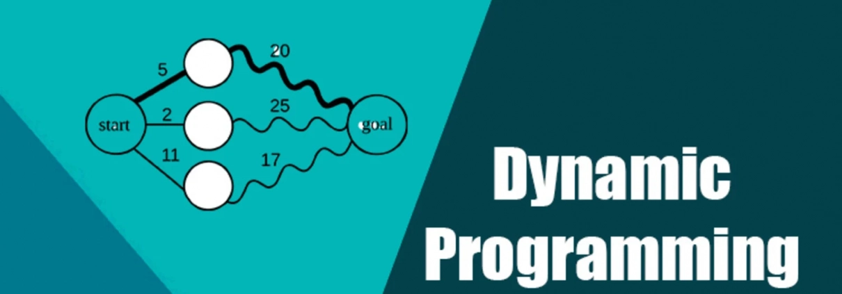
Dynamic Programming (DP) is a powerful technique in computer science and mathematics used to solve a wide range of optimization and combinatorial problems. It’s a method that involves breaking down complex problems into simpler overlapping subproblems, solving each subproblem only once, and storing the results to avoid redundant calculations. This approach greatly improves the efficiency of algorithms and can be applied to various domains, including algorithms for optimization, sequence alignment, and more.

In this comprehensive guide, we’ll explore the fundamental concepts of dynamic programming, provide intuitive explanations, and offer code examples in Python to illustrate how DP can be applied to solve real-world problems.

What is Dynamic Programming?

Dynamic Programming is a method for solving problems by breaking them down into smaller subproblems, solving each subproblem only once, and storing the results in a table or memoization data structure. When a subproblem is encountered again, instead of recalculating its solution, we look up the previously computed result, leading to significant time savings.

The term “programming” in dynamic programming has nothing to do with coding but comes from the word “pro-gramme”, which means a plan or a set of rules. It was coined by Richard Bellman in the 1950s when he was working on optimization problems. Dynamic Programming provides a structured way to find optimal solutions to problems with overlapping subproblems, and it is particularly useful when a problem can be broken down into smaller, similar subproblems.

Key characteristics of dynamic programming:

Optimal Substructure: The problem can be divided into smaller subproblems and the optimal solution to the original problem can be constructed from the optimal solutions of its subproblems.
Overlapping Subproblems: The same subproblems are solved multiple times in a recursive manner. Dynamic Programming stores the results of these subproblems to avoid redundant computation.

Fibonacci Sequence: A Simple DP Example

To grasp the concept of dynamic programming, let’s start with a classic example: calculating the Fibonacci sequence. The Fibonacci sequence is defined as follows:

F(0) = 0
F(1) = 1
F(n) = F(n-1) + F(n-2) for n > 1

We can calculate Fibonacci numbers using recursion, but this approach leads to an exponential number of function calls and is highly inefficient for large `n`. Dynamic programming offers a more efficient solution by avoiding redundant calculations.

Here’s a Python code snippet for calculating Fibonacci numbers using dynamic programming:

def fibonacci_dp(n):
    fib = [0] * (n + 1)

    # Base cases
    fib[0] = 0
    fib[1] = 1

    # Calculate Fibonacci numbers from 2 to n
    for i in range(2, n + 1):
        fib[i] = fib[i - 1] + fib[i - 2]

    return fib[n]

# Example usage
n = 10
print(f"Fibonacci({n}) =", fibonacci_dp(n)) # Output: Fibonacci(10) = 55

In this code, we create an array `fib` to store the Fibonacci numbers. We start by initializing the base cases (`F(0)` and `F(1)`) and then use a loop to calculate Fibonacci numbers from `2` to `n` by summing the previous two values. This way, we avoid redundant calculations, and the time complexity is reduced from exponential to linear (`O(n)`).

Types of Dynamic Programming

Dynamic Programming can be categorized into two main types:

Top-Down (Memoization): In the top-down approach, we start with the original problem and recursively break it down into smaller subproblems. We use a memoization table (usually an array or dictionary) to store the results of already solved subproblems. When a subproblem is encountered, we first check if its solution is in the memoization table. If not, we calculate it and store the result, which can be looked up in future recursive calls.
Bottom-Up (Tabulation): In the bottom-up approach, we start with the smallest subproblems and iteratively build up the solution to the original problem. We use a table or array to store the results of subproblems and fill it in a specific order, typically from the smallest subproblems to the largest. This approach is more efficient in terms of space complexity since we only need to store results for the necessary subproblems.

Both approaches are equivalent and can be used interchangeably, but tabulation is often preferred when it’s straightforward to determine the order in which subproblems should be solved.

Longest Common Subsequence (LCS): A Practical DP Example

Let’s explore a more practical example of dynamic programming: finding the Longest Common Subsequence (LCS) between two sequences. Given two sequences, the LCS is the longest sequence that appears as a subsequence in both sequences. For example, given the sequences “ABCD” and “ACDF,” the LCS is “ACD”.

Here’s a Python code snippet for finding the LCS using dynamic programming:

def longest_common_subsequence(X, Y):
    m = len(X)
    n = len(Y)

    # Create a 2D table to store LCS lengths
    dp = [[0] * (n + 1) for _ in range(m + 1)]

    # Build the dp table
    for i in range(1, m + 1):
        for j in range(1, n + 1):
            if X[i - 1] == Y[j - 1]:
                dp[i][j] = dp[i - 1][j - 1] + 1
            else:
                dp[i][j] = max(dp[i - 1][j], dp[i][j - 1])

    # Reconstruct the LCS
    lcs = []
    i, j = m, n
    while i > 0 and j > 0:
        if X[i - 1] == Y[j - 1]:
            lcs.append(X[i - 1])
            i -= 1
            j -= 1
        elif dp[i - 1][j] > dp[i][j - 1]:
            i -= 1
        else:
            j -= 1

    return ''.join(reversed(lcs))

# Example usage
X = "AGGTAB"
Y = "GXTXAYB"
print("Longest Common Subsequence:", longest_common_subsequence(X, Y))

In this code, we create a 2D table `dp` to store the lengths of LCS for different prefixes of the input sequences `X` and `Y`. We iteratively fill the table by comparing characters from both sequences. If characters match, we increment the length by 1; otherwise, we take the maximum of the LCS lengths from the previous rows and columns. Finally, we backtracked from the last cell to reconstruct the LCS.

Coin Change Problem: An Optimization Challenge

Another classic dynamic programming problem is the Coin Change Problem. Given a set of coin denominations and a target amount, the task is to find the minimum number of coins required to make up the target amount. This problem demonstrates how dynamic programming can be used for optimization.

Here’s a Python code snippet to solve the Coin Change Problem using dynamic programming:

def min_coins(coins, target):
    # Initialize a table to store minimum coin counts
    dp = [float('inf')] * (target + 1)
    dp[0] = 0

    # Calculate minimum coin counts for all amounts from 1 to target
    for amount in range(1, target + 1):
        for coin in coins:
            if coin <= amount:
                dp[amount] = min(dp[amount], dp[amount - coin] + 1)

    return dp[target] if dp[target] != float('inf') else -1

# Example usage
coins = [1, 2, 5]
target = 11
print("Minimum coins required:", min_coins(coins, target))

In this code, we create an array `dp` to store the minimum coin counts for different amounts from `0` to `target`. We initialize the table with infinity except for `dp[0]`, which is set to `0` because no coins are needed to make up zero. We then iterate through all possible amounts and coins, updating the minimum coin counts as we find better solutions. Finally, we return the minimum coin count for the target amount or `-1` if it’s impossible to make the amount with the given coins.

When to Use Dynamic Programming

Dynamic Programming is a powerful technique for solving a wide range of problems, but it’s not always the best choice. Here are some factors to consider when deciding whether to use dynamic programming:

Optimal Substructure: The problem can be broken down into smaller subproblems with the same characteristics.
Overlapping Subproblems: The same subproblems are solved multiple times, leading to redundant computation.
Memoization or Tabulation: Decide whether to use the top-down (memoization) or bottom-up (tabulation) approach based on problem requirements and simplicity.
Time Complexity: DP often reduces the time complexity of problems from exponential to linear or polynomial.
Space Complexity: Consider memory requirements when choosing between memoization and tabulation.
Simplicity: Sometimes, simpler algorithms (e.g., greedy algorithms) may suffice for the problem at hand.

Conclusion

Dynamic Programming is a versatile and powerful technique for solving a wide variety of problems efficiently by breaking them down into smaller subproblems and avoiding redundant calculations. Through this guide, we’ve explored the fundamental concepts of dynamic programming, including optimal substructure and overlapping subproblems, and seen practical examples of how to implement dynamic programming solutions in Python.

As you dive deeper into dynamic programming, you’ll encounter more complex problems and variations of the technique. However, the core principles discussed here will remain valuable in understanding and implementing DP solutions effectively. Whether you’re working on algorithmic challenges or real-world optimization problems, dynamic programming can be a valuable tool in your problem-solving toolkit.

0 0 votes

Article Rating