Greedy Algorithms: Principles and Practical Applications

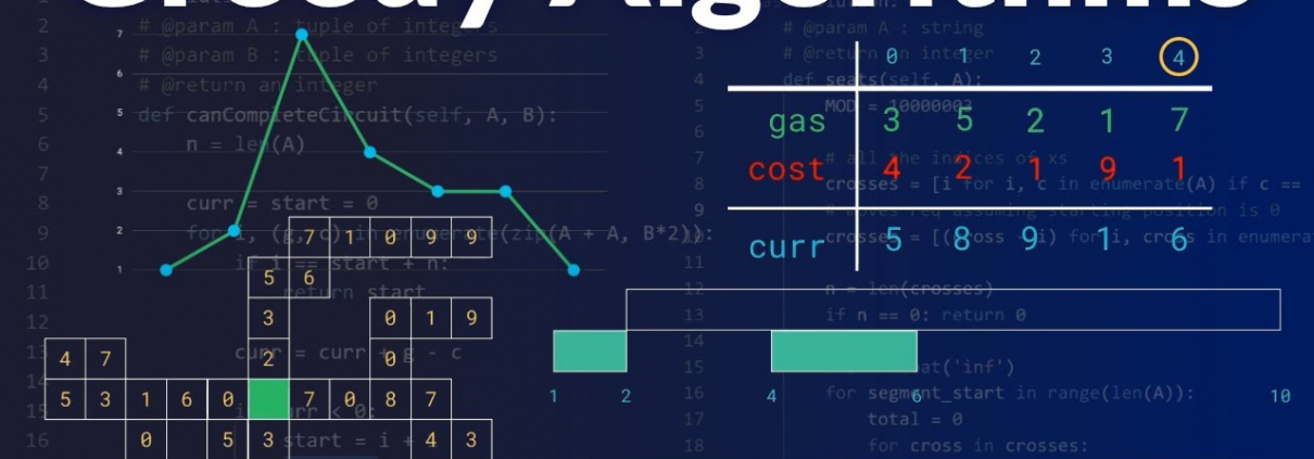
Greedy algorithms are a fundamental concept in computer science and mathematics, often employed to solve optimization problems by making locally optimal choices at each step. These algorithms are renowned for their simplicity and efficiency, making them an indispensable tool in various domains, including computer science, economics, and engineering. In this article, you’ll delve into the principles of greedy algorithms, explore their characteristics, and provide practical code examples to illustrate their application.

What are Greedy Algorithms?

A greedy algorithm is an approach to problem-solving that makes a series of choices, one at a time, with the goal of reaching an optimal solution. At each step, a greedy algorithm selects the best available option based on some predetermined criteria, without considering the global context or potential consequences of the choice in future steps. The key principle is to always make the locally optimal choice, hoping that the cumulative effect of these choices will lead to the best overall solution.

The term “greedy” implies that the algorithm exhibits a selfish behavior, always prioritizing the option that seems most advantageous at the moment, without considering the big picture. This characteristic simplifies the design and analysis of greedy algorithms, but it also introduces the risk of ending up with suboptimal or even incorrect solutions.

Characteristics of Greedy Algorithms

To understand and effectively utilize greedy algorithms, it’s essential to recognize their primary characteristics:

Greedy Choice Property

At each step of the algorithm, a greedy algorithm makes a choice that appears to be the best option at that moment. This choice is typically based on some objective function or criteria. The algorithm doesn’t consider future consequences; it only focuses on the immediate decision.

Optimal Substructure

Greedy algorithms often possess the optimal substructure property, which means that an optimal solution to the overall problem can be constructed from optimal solutions to its subproblems. This property simplifies the problem-solving process by allowing the algorithm to work incrementally.

Lack of Backtracking

Greedy algorithms usually don’t backtrack or reconsider previous choices. Once a decision is made, it’s final. Consequently, the algorithm’s efficiency and simplicity often come at the cost of potentially missing globally optimal solutions.

Greedy Algorithms May Not Always Be Optimal

While greedy algorithms work well for many problems, they do not guarantee finding the globally optimal solution for all problems. In some cases, they may lead to suboptimal solutions.

Common Applications of Greedy Algorithms

Greedy algorithms are widely used in a variety of real-world applications. Let’s explore some common scenarios where they excel:

1. Minimum Spanning Tree (MST)

Problem: Given a connected, undirected graph with edge weights, find the minimum spanning tree, a subgraph that includes all vertices with the minimum possible total edge weight.
Greedy Approach: Kruskal’s or Prim’s algorithm selects edges with the lowest weights while ensuring that no cycles are formed.

# Kruskal's Algorithm in Python
from heapq import heapify, heappop, heappush

def kruskal(graph):
    minimum_spanning_tree = []
    heapify(graph['edges'])
    parent = {vertex: vertex for vertex in graph['vertices']}

    while graph['edges']:
        weight, u, v = heappop(graph['edges'])
        if parent[u] != parent[v]:
        minimum_spanning_tree.append((u, v, weight))
        old_parent, new_parent = parent[u], parent[v]
        for vertex, p in parent.items():
        if p == old_parent:
        parent[vertex] = new_parent

    return minimum_spanning_tree

2. Huffman Coding

Problem: Compress a message by assigning variable-length codes to characters to minimize the total encoded message length.
Greedy Approach: Huffman coding assigns shorter codes to more frequent characters, resulting in efficient compression.

# Huffman Coding in Python
import heapq

def build_huffman_tree(data):
    heap = [[weight, [char, ""]] for char, weight in data.items()]
    heapq.heapify(heap)

    while len(heap) > 1:
        lo = heapq.heappop(heap)
        hi = heapq.heappop(heap)
        for pair in lo[1:]:
            pair[1] = '0' + pair[1]
        for pair in hi[1:]:
            pair[1] = '1' + pair[1]
        heapq.heappush(heap, [lo[0] + hi[0]] + lo[1:] + hi[1:])

    return sorted(heapq.heappop(heap)[1:], key=lambda p: (len(p[-1]), p))

3. Fractional Knapsack

Problem: Given a set of items with weights and values, determine the most valuable combination of items to fit into a knapsack of limited capacity.
Greedy Approach: Select items with the highest value-to-weight ratio until the knapsack is full.

# Fractional Knapsack in Python
def fractional_knapsack(items, capacity):
    items.sort(key=lambda x: x[1] / x[0], reverse=True)
    total_value = 0.0
    knapsack = []

    for item in items:
        if item[0] <= capacity:
            knapsack.append(item)
            total_value += item[1]
            capacity -= item[0]
        else:
            fraction = capacity / item[0]
            knapsack.append((item[0] * fraction, item[1] * fraction))
            total_value += item[1] * fraction
            break

    return knapsack, total_value

4. Dijkstra’s Shortest Path

Problem: Find the shortest path from a source node to all other nodes in a weighted graph.
Greedy Approach: At each step, select the unvisited node with the smallest tentative distance and update its neighbors’ distances.

# Dijkstra's Algorithm in Python
import heapq

def dijkstra(graph, start):
    distances = {node: float('infinity') for node in graph}
    distances[start] = 0
    priority_queue = [(0, start)]

    while priority_queue:
        current_distance, current_node = heapq.heappop(priority_queue)

        if current_distance > distances[current_node]:
            continue

        for neighbor, weight in graph[current_node].items():
            distance = current_distance + weight
            if distance < distances[neighbor]:
                distances[neighbor] = distance
                heapq.heappush(priority_queue, (distance, neighbor))

    return distances

Advantages and Limitations of Greedy Algorithms

Advantages:

Greedy algorithms are relatively easy to understand and implement.
They often provide efficient solutions to problems.
They are suitable for problems that exhibit the greedy choice property.

Limitations:

Greedy algorithms do not always guarantee an optimal solution.
The choice of the greedy criterion can greatly impact the result.
They may not work well for problems with complex constraints or when global optimization is required.

Conclusion

Greedy algorithms are a powerful and versatile tool for solving optimization problems. While they come with the risk of not always producing globally optimal solutions, their simplicity and efficiency make them valuable in a wide range of applications. Understanding the greedy choice property, optimal substructure, and the absence of backtracking is crucial when designing and analyzing these algorithms. Whether you’re working on finding minimum spanning trees, data compression, knapsack problems, or shortest path algorithms, the principles of greedy algorithms offer an elegant and practical approach to problem-solving.

0 0 votes

Article Rating